Next week I will be co-presenting a paper at the APEE conference on the reliability of historical estimates of income inequality in the United States. Our paper examines and offers a number of corrections to the widely cited income inequality time series by Thomas Piketty and Emmanuel Saez (2003). This series provides the baseline for multiple subsequent studies of inequality, and is the primary U.S. inequality series in the World Wealth & Income Database.
The Piketty-Saez series is the primary example of the famous U-shaped inequality trend line for the United States in the 20th century that was prominently featured in Piketty’s 2014 book Capital in the 21st Century. It is calculated using income tax records from the IRS and a variety of complex statistical techniques to extract a distributional measure of income inequality for the top 1% through top 10% of income earners.
In this post I want to focus specifically on how Piketty & Saez arrive at their estimates for the pre-World War II period, or basically the first half of their U-shape. This period is both interesting and statistically problematic because the IRS data they use as their source has several under-recognized drawbacks. Most American households were not eligible to pay income taxes prior to a rapid expansion of the tax base through new wartime income tax laws in 1941-1945. Before 1941, only about 10% of U.S. households – or even fewer in some years – were required to file their income taxes. In addition, tax enforcement was often deeply inconsistent in those early years, resulting in ample opportunities for both illegal tax evasion and legal tax avoidance. There were even year-to-year inconsistencies in the accounting measurements that the IRS employed to tabulate reported income. Piketty & Saez are aware of some of these issues and attempt to adjust for them (e.g. IRS accounting issues), but also largely inattentive to others (e.g. evasion and avoidance problems). Our paper argues that the cumulative effect of these issues renders their pre-World War II data, or basically the first half of the U-shape, unusable.
I will be detailing several of these issues in the coming months, but today I’ll be walking you through some of the issues with one of the most dramatic adjustments that Piketty and Saez make. To reach their initial income distributions for the pre-war period, they begin by taking raw filing data from the IRS’ annual Statistics of Income (SOI) report (most of their post-war data comes from more comprehensive IRS microfile sources that are only available from the 1960s to the present). They use the SOI to calculate distributional estimates using a Pareto interpolation technique that is discussed at length in their paper’s data appendix. The technique itself is fairly standard fare, assuming the source data are accurate. Due to some of the aforementioned problems of IRS accounting inconsistencies and the low number of eligible tax filers before the war, they have to make a few adjustments to its results.
It’s easiest to see the effects of the adjustments they make through 3 steps in the chart below (showing the calculations for the top 10% income share):
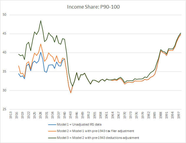
Model 1, in blue, shows the raw Pareto interpolation from the unadjusted IRS SOI reports. Model 2, in red, attempts to address the problem of insufficient returns due to the low number of eligible tax filers before World War II. To do so it estimates and integrates a modest number of “missing returns” by taking the ratio of married vs. single tax filers in the pre-war years. As you can see, it increases the distributional share of the top 10% slightly before 1940. It does not alter any of the post-1940 results.
A much larger adjustment comes from what we describe as Model 3, shown here in dark green. This is an accounting adjustment that purports to address the IRS’ switch from Net Income (NI) to Adjusted Gross Income (AGI) in 1943-1944. The difference between the two involves how each handle deductions for charitable giving, local and state tax payments, and some categories of interest payment. It is strictly a feature of the way the tax code handled each. AGI encompasses a share of untaxed but realized income that isn’t present in NI, hence the justification for making an adjustment.
A problem emerges though with how Piketty and Saez calculate this NI-to-AGI adjustment for Model 3. As you can see in the chart above, the Model 3 adjustments are the most substantial change that Piketty and Saez make to the pre-World War II Pareto calculations. They consistently add about 5 percentage points to the distributional share before 1941, but relatively little thereafter.
The way that Piketty and Saez go about calculating this adjustment is, unfortunately, opaque. Using their calculation files to replicate the adjustment, it appears that they simply inserted an even, constant, and nicely rounded multiplier across the pre-war income share. The multiplier in turn “bumps” the entire trendline upward until World War II, when Piketty and Saez begin relaxing their multipliers and then bottoming them out to zero with the 1943-1944 NI to AGI switch at the IRS. The weights that Piketty and Saez use for their multipliers are highlighted in blue on their spreadsheet below. The yellow highlighted cells reflect the post-AGI switch at the IRS.
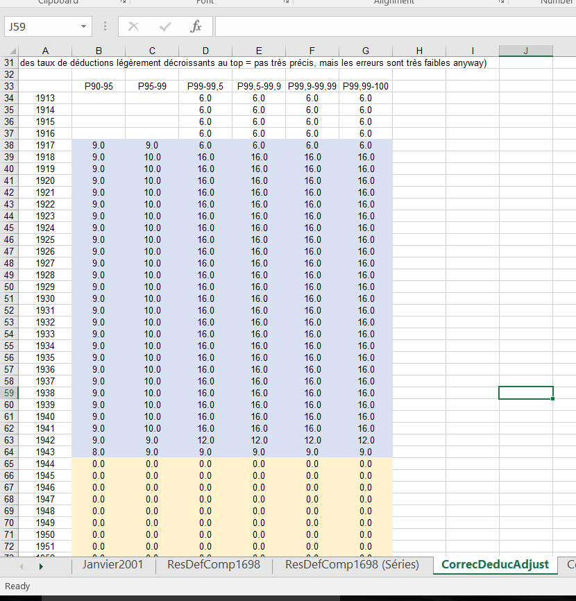
Notice that all of the adjustments are even, rounded numbers. Also notice two important features: (1) the weights they apply scale upward toward the highest income earning percentiles and (2) the weights are held perfectly constant across the board from 1918 to 1941, and then rapidly reduced from 1941 to 1943. This presumably reflects a number of assumptions that Piketty & Saez make, including the effects of the wartime expansion of the tax base that occurred with a succession of tax hikes after 1940. They also very conveniently create a shape in the resulting time series that looks like the first half of the famous U-shaped pattern.
Piketty and Saez provide very little indication of where any of these weights even come from, let alone if they accurately reflect the size and distribution of untaxed deductions from the pre-AGI period of IRS accounting. The evenly rounded and constant numbers also strongly suggest that simple “guesstimation” is at play (my readers will remember that Piketty has a bad habit of guesstimating numbers and weights along these lines in historical periods of sparse or insufficient data, usually to create the trend line shape that he wishes to depict).
Part of the problem comes from the unavoidable issue of insufficient historical data. The IRS records are not sufficiently complete to perform a direct NI-to-AGI adjustment in most pre-war years. The question then becomes one of whether the Piketty-Saez weights, apparently guesstimated, are justifiable. Let me offer one piece of evidence that strongly suggests they are not. While the IRS did not report or differentiate all types of deductions in the pre-war period, they did track tax-exempt donations to charities from the mid 1920s onward.
Annual charitable deduction totals fluctuated wildly throughout this period, showing deep responsiveness to changes in the tax code and to the Great Depression. The inflation-adjusted totals are depicted below:
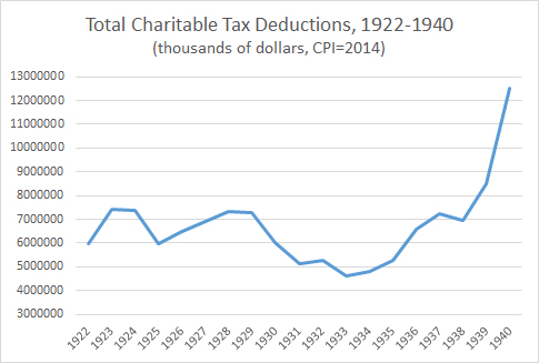
Charitable deductions represent only a part of the NI-to-AGI adjustment, so we cannot make a direct 1-to-1 claim about their effects. Still, the severity of the fluctuations itself suggests at least one strong reason why the stable, constant multiplier that Piketty and Saez employ could be highly problematic.
This is but one of many similar issues I will be highlighting with their pre-World War II adjustments in the forthcoming paper and future posts. It is a substantial one though, the removal of which completely alters and substantially diminishes the first half of their famous U-shaped distribution.