If you’ve been following the news for the past few days you’ve probably seen a reference to the Financial Times’ investigation of the data behind Thomas Piketty’s recent bestseller Capital in the 21st Century. While it is difficult to extrapolate intentions from data alone, it seems safe to say now that Piketty was – at minimum – sloppy with his data analysis. His time series work on historical indexes of wealth inequality in particular seems to be riddled with erroneous transcriptions, amateurish weighting and formula assumptions, and a casual cherrypicking of data.
Several people have already gone to great lengths to analyze what these errors mean for his overall arguments. While I’ll leave that discussion to others, I’d like to call attention to one specific curiosity in Piketty’s work as it pertains to purported wealth inequality data for the United States and, specifically, what appears to be a clear cherrypicked manipulation of data sources.
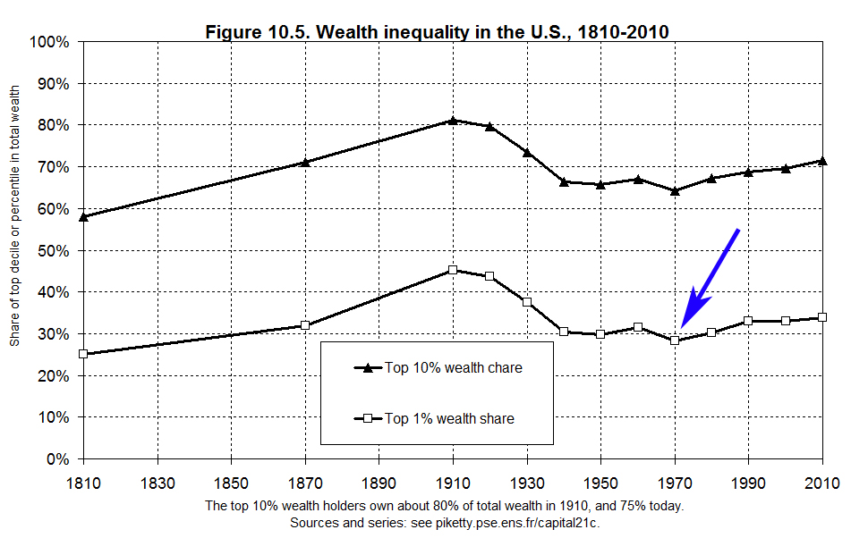
The following is Figure 10.5, which shows Piketty’s estimate of wealth inequality in the United States. The graph shows estimates for both the top 10% and top 1%, the latter of which I’ve highlighted with the blue arrow.
A couple of observations about this graph:
1. His data prior to 1910 is sporadic and really consists of only two datapoints, which are meant as historical estimates for a century’s time during which Piketty simply does not have consistent reliable data. Make of that what you will about the implications of this graph for anything before 1910, but for purposes of this discussion we may ignore it and focus on 1910-2010, where the data seems more robust.
2. The quick interpretation of Piketty’s data for 1910-2010 is that US wealth inequality, which was near or at a peak a century ago, dipped dramatically in the mid 20th century yet since circa the 1970s it has been on the rebound.
3. Note that Piketty’s chart has only 10 data points for the century in question. This is because he is presenting decennial averages for wealth distributions rather than raw data. The averaging technique from which he derived these numbers may be found in the worksheet TS10.1DetailsUS on this spreadsheet.
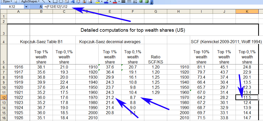
Turning next to worksheet TS10.1DetailsUS, we find Piketty’s sources and decennial averaging techniques. Specifically, the core of his data came from a larger time series of wealth holdings for the top 1% in the US as estimated by Kopczuk and Saez – the latter his sometimes-collaborator. (The Kopczuk-Saez dataset was the basis of several articles in the early 2000s and may be accessed in this 2004 study in the National Tax Journal). Piketty then uses the Kopczuk-Saez data to calculate decennial averages for the top 1% of wealth in the US, which he then merges with another data source and indexes to a “corrective” multiplier that slightly increases the decennial averages he calculated from the Kopczuk-Saez set.
One thing to note about Kopczuk-Saez at this point is that their time series, covering 1916 to 2000, has many gaps and only presents data for 64 out of the 84 years that are included in their study’s scope. This is not necessarily a problem in itself, but it does begin to become distortive when they are used to calibrate a decennial average and then conduct cross-decade comparisons between the results – which is exactly what Piketty did.
The distribution of the gaps in the Kopczuk-Saez dataset is very uneven. Specifically, the number of data points by decade are as follows:
1910s: 4
1920s: 10
1930s: 10
1940s: 10
1950s: 5
1960s: 4
1970s: 2
1980s: 8
1990s: 10
2000s: 1
Out of this sporadic compilation, Piketty takes his decennial averages for 1910s-1950s and 1970s from Kopczuk-Saez, and then recalibrates them upwardly. The 1960s data is a modified combination of Kopczuk-Saez and another supplemental data set. 1980s-2000s then draw from two other supplemental data sets based on the Survey of Consumer Finances, including a 2010 addition to the available data.
While fully recognizing that historical data sources are often incomplete and less than ideal for this type of analysis, Piketty’s mishmash of sources and his chosen averaging technique to get around the point of a major data gap is…well…very odd.
These gaps are not necessarily a basis to consarn his entire data set or the sources it draws from into interpretive uselessness, but they do create a strangely uneven basis for calculating a summary of their sporadic contents through decennial averaging.
All of that stated briefly, the low point for wealth concentration on Piketty’s chart (see the upward kink after the 1970s datapoint on Figure 10.5 above), and the point at which a supposed reversal in US wealth concentration trends begins, also corresponds to the period of the biggest decennial data gap in the Kopczuk-Saez data set. Despite this deficiency, Piketty’s 1970s average (again, based on only 2 data points in a decade that was also particularly notorious for its business cycle turmoil and economic fluctuation) is presented with a weight no different from prior decades in the 20th century where 10 full years of estimated data is readily available, or from subsequent decades where he switches, at least in part, to more complete supplemental data sets.
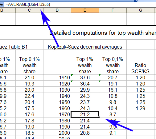
Note the data points in the blue box below. These two slim estimations are the genesis of Piketty’s decennial average for the entire 1970s, which also happens to be bottoming out for wealth accumulation among the super-rich and the turning point of his much-vaunted claims about subsequent inequality trends. By comparison, his averages for earlier decades include as many as 10 years worth of highly fluctuating data:

But there’s something further to consider. The Kopczuk-Saez raw estimates also diverge fairly substantially from the results of Piketty’s decennial averaging technique.
There are two reasons for this. One of them is a plausibly debatable point of data calibration and concerns whether the Kopczuk-Saez study underestimates wealth distribution across the categories included. To this end Piketty, as previously noted, upwardly recalibrates their numbers (albeit somewhat casually) in a way that adds between roughly 6 and 12 percentage points to the wealth holdings of the top 1%, depending on the decade. Since Piketty’s top 1% averages are then used to calibrate and indeed create his decennial estimates for the top 10% (which were not a part of the original Kopczuk-Saez data set), this modification – plus a couple of tweaks brought in from two successive studies – also carries over to that larger set of figures as well.
The second begins to highlight the problems created by the uneven and sporadic distribution of source data that I just mentioned when Piketty constructs his decennial averages. By converting unevenly distributed root estimates into an evenly distributed decennial average, he ends up artificially creating a very pronounced “kink” in his Figure 10.5 with a clear downward trend predating it and an equally clear upward trend emerging from it over the next three decades. The political implication, of course, is that the unequal distribution of wealth in the United States is undergoing a consistent and uninterrupted rise towards levels unseen since at least the 1930s and will presumably continue beyond.
Contrast that with the yearly raw source data from which Piketty’s chart (at least through the 1970s, and then modified thereafter with supplemental sets) is directly derived and recalibrated. The aforementioned 1970s gap is readily evident, with no means of determining whether a the seemingly sharp drop in 1976 was in fact sustained throughout the sizable data gaps to either side of it, or to what extent it accurately captures the decennial figure Piketty then extracts for the 1970s.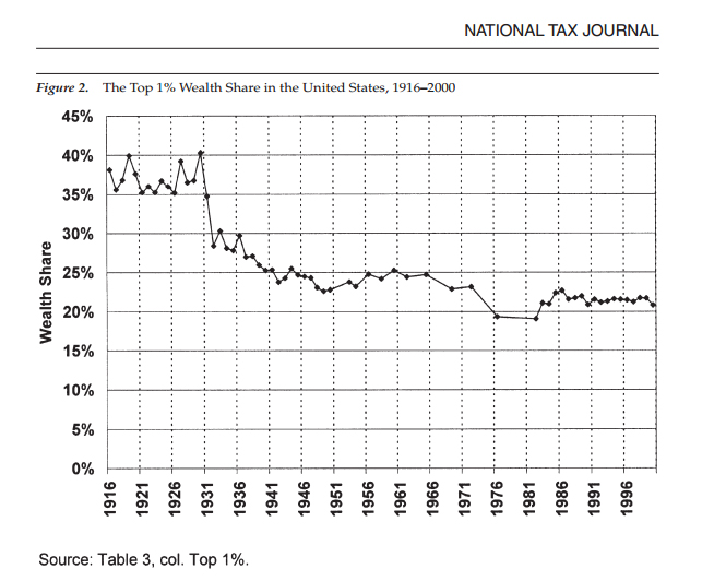
What we therefore seem to have in Figure 10.5 is less a synthesis of other data sets, or even an update of their numbers using newer data, than a sloppy muddying of the water around them by actually reducing the precision of yearly data into decennial summary terms of inexplicably equal weight, given the data gaps, and then the projection of artificial trend lines upon them under the guise of “smoothing” and recalibration.
While this seems to be more a product of sheer sloppy stats work than willful deceit, it is also not coincidental that his slipshod averaging techniques yielded a product that was consistent with his political message or that, upon finding that it hit desirable political notes, that product was put into print by a major academic press despite serious issues with the rigor of its analysis.